Types of Forces
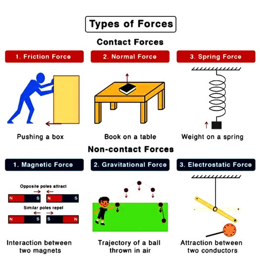
- Contact Forces: These forces occur when two objects are physically touching each other. Examples include friction, tension, normal force, and applied force.
- Non-Contact Forces: These forces act over a distance without physical contact. Examples include gravitational force, electromagnetic force, and nuclear forces.
Newton's Laws of Motion
Along with calculus, Newton also essentially invented modern physics, starting with his three laws of motion. Before Isaac Newton, the understanding of motion was limited and often incorrect. Newton's laws provide a framework for understanding how forces affect the motion of objects.
In his book, Principia Mathematica, Newton laid out his three laws of motion:
- First Law (Inertia): An object at rest stays at rest and an object in motion stays in motion with the same speed and in the same direction unless acted upon by an unbalanced force.
- Second Law \(\vec{F}=m\vec{a}\): The acceleration of an object depends on the net force acting on it and its mass. This is expressed as F = ma, where F is the net force, m is the mass, and a is the acceleration.
- Third Law (Action-Reaction): For every action, there is an equal and opposite reaction.
First Law of Motion (Inertia)
The first law, also known as the law of inertia, states that an object will remain at rest or in uniform motion unless acted upon by an external force. This means that if no net force is acting on an object, its velocity will not change. This law highlights the concept of inertia, which is the tendency of objects to resist changes in their state of motion.
There's a running joke where most people say that Newton's first law just states that a stationary object stays still. But it goes a bit deeper, it talks of inertia and resistance to changes in motion. This law is often overlooked because it seems so obvious, but it's actually quite profound. It appears in some parts of physics unrelated to forces and even on nonphysical systems such as the stock market.
We call this the law of inertia because inertia is defined to be an object's resistance to changes. For resistance to linear motion, we have mass. For resistance to rotational motion, we have what we call the moment of inertia which we'll discuss later.
Second Law of Motion (\(\vec{F}=m\vec{a}\))
The second law of motion quantifies forces and their effects on the motion of objects. It states that the acceleration of an object is directly proportional to the net force acting on it and inversely proportional to its mass. This relationship is expressed mathematically as the famous equation: \[\vec{F}=m\vec{a}.\]
With this one equation, we can understand how forces affect motion and predict the behavior of objects under various conditions. It allows us to convert physical systems into a mathematical model called a differential equation.
Differential equations: a handy tool
Differential equations are equations that involve the derivatives of a function. The perfect example is Newton's second law \(\vec{F}=m\vec{a}\), which relates the acceleration (2nd derivative of position with time) of an object to the net force (possibly a function of position time and velocity) acting on it.
Examples of differential equations from Newton's second law may include:
- \(\frac{d^2x}{dt^2}=-mg\) (Free fall)
- \(\frac{d^2x}{dt^2} = -\frac{k}{m}x\) (Simple harmonic oscillator)
- \(\frac{d^2x}{dt^2} = -\frac{GM}{x^2}\) (Gravitational attraction)
- \(\frac{d^2x}{dt^2} = -c \frac{dx}{dt}\) (linear fluid drag)
Each of these differential equations require different techniques to solve them. We will not cover all these different types of techniques in here. Instead, we will use what is called an Anzatz, which is just a fancy way for saying guess.
As a nice application of what we just gone through, consider the following problem:
Simple harmonic oscillator
We can model the force which a spring exerts on an object as \(\vec{F} = -k\vec{x}\), where \(k\) is called the spring constant and \(\vec{x}\) is the displacement from equilibrium (where the spring is at rest or unstreched).
It can be seen in the applet that the spring here will oscillate. Playing around with the simulation here, you can find that increasing the spring constant increases the frequency of oscillation, so does decreasing the mass on the spring. But why is this true?
to uncover how the mass of the object and the spring constant affects the frequency of the oscillation, we must use Newton's second law. We have that the net force on the object is given by \[\vec{F} = m\vec{a}.\] But we also know that the only force acting on the object is the spring force, so we can find that \[-k\vec{x} = m\vec{a}.\] Rearranging this gives \[\vec{a} = -\frac{k}{m}\vec{x}.\]
If we set the acceleration equal to the second derivative of position, we get a differential equation (equation that involves derivatives) that describes the motion of the spring. This differential equation is \[\frac{d^2x}{dt^2} = -\frac{k}{m}x.\]
Hm, now we need to find a solution to this equation. It says that the second time derivative of \(x\) with respect to time is equal to \(-\frac{k}{m}x\). It is proportional to the negative of itself.
This is very similar to what we saw in uniform circular motion. In there we saw that the acceleration of an object in uniform circular motion was proportional to the negative of its position vector. The solution to that was a sine or cosine function. So we can guess that the solution to this differential equation is also a sine or cosine function. Let's try \[x(t) = A\cos(\omega t + \phi)\] where \(A\) is the amplitude, \(\omega\) is the angular frequency, and \(\phi\) is the phase constant.
Plugging this into the equation lets us find that the solution is valid when \[\omega = \sqrt{\frac{k}{m}}=2\pi f.\] where \(f\) is the frequency of oscillation.
Therefore, we have found that the frequency of oscillation of a mass-spring system is given by \[f = \frac{1}{2\pi}\sqrt{\frac{k}{m}}.\] This shows that increasing the spring constant \(k\) increases the frequency, while increasing the mass \(m\) decreases the frequency, which matches our observations from the simulation.
There we have it, our first differential equation! Along with that, this is the first time we come across the harmonic oscillator. We will (maybe not so soon) learn that this will essentially become our best friend in other parts of physics such as quantum mechanics, quantum field theory and analytic mechanics.
Third Law of motion
Finally, we have the third law of motion. It states that for every force applied, there is an equal and opposite reaction. This is why punching rocks hurt us more than it damages them. This is how objects are able to lie idly on tables.
We do not exactly represent Newton's third law as an elegant mathematical equation like the second law. It is instead better to see it in action through what we call free body diagrams.
Free body diagrams
Consider a book at rest on a table. What a free body diagram does is that it isolates the object of interest (the book) and shows all the forces acting on it. It is a very handy tool when coming across problems in forces.
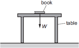
It may seem tempting to just say that the book has only 1 force acting on it, which is the gravitational force (\(\vec{w}\)) pulling it downwards. However, if we used Newton's second law, we find that this should be completely wrong as the book would just be falling through the table with nothing preventing it from falling down.
To resolve this problem, we invoke Newton's third law. As the book clearly must be exerting a force onto the table, the table must also be exerting a force back on the book. This upward force is called the normal force (\(\vec{N}\)). The normal force balances the weight of the book, keeping it at rest.
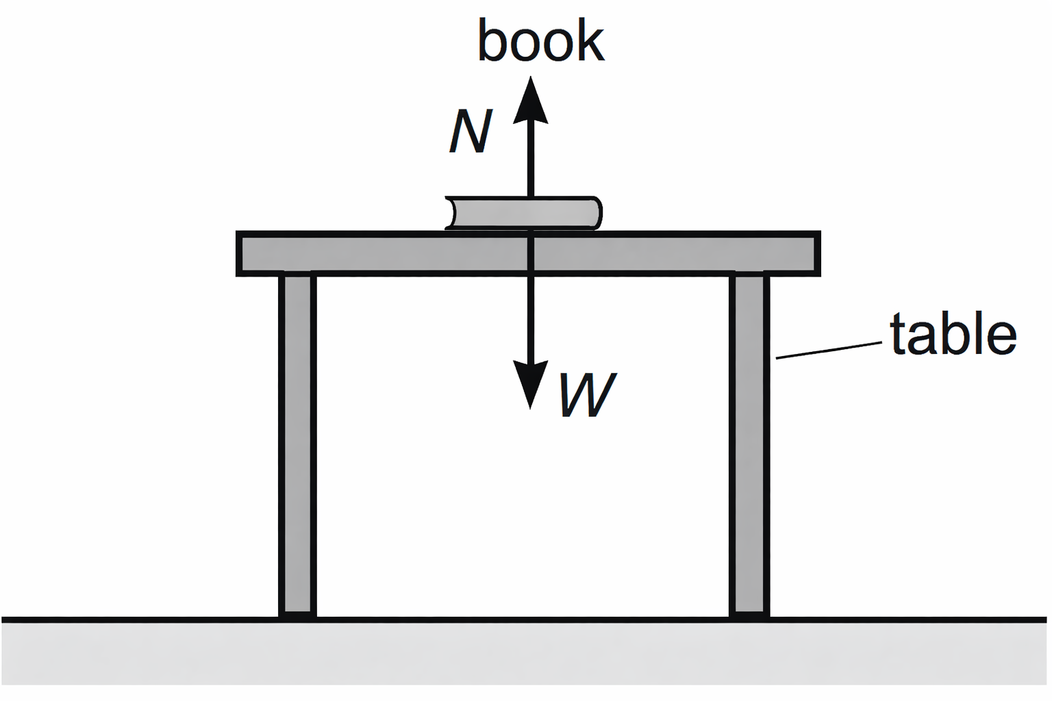
This looks better. As the book shouldn't be falling through the table, the normal force completely negates the weight force, making the net force \(0\) and the book stationary.
Rotational dynamics and the moment of inertia
Similar to what we did in the previous section, we can also try to recreate what we had above for rotations
Before doing so, we need a few mathematical tools which won't seem very obvious yet.
Vector products: dot and cross product of vectors
In the previous section we made use of vectors to describe physical quantities such as position and velocity. They follow nice rules, you can add them together and multiply them by scalars to stretch them. But what if we tried to multiply a vector with another vector?
Athough in usual vector arithmetic we can add and subtract vectors, multiplying vectors isn't as straightforward. Do we get a vector from multiplying them or do we get a scalar? The answer is both.
Because of this problem 2 famous types of multiplications were made, the cross product and the dot product. The first generates another vector whist the other generates a scalar.
Let's take a look at the cross product first:
Cross product
This is the vector product which generates another vector. This is denoted by the symbol \(\times\). So we can say that if \[\vec{C} = \vec{A} \times \vec{B}\] Then \(\vec{C}\) is the cross product of \(\vec{A}\) and \(\vec{B}\).
That's neat and all but if the result of a product of 2 vectors is another vector, what direction must it have? The direction of the cross product is perpendicular to both vectors involved in the product. The direction of the cross product can be determined by the right-hand rule.
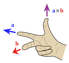
Very nice, we have made the direction of the cross product clear. However, remember that a vector is a quantity with both magnitude and direction. The cross product of two vectors is a vector perpendicular to both of the original vectors, But what about it's magnitude?
Intuitively, we want the cross product to be defined for all 3d vectors. But what happens if both vectors point in the same direction? What direction should the cross product point then? An easy way to resolve this is to just say that if the 2 vectors are parallel, it's cross product will be the \(0\) vector.
Another point we can make is if this really is a type of multipication, then the larger the magnitudes of the vectors are, the bigger the cros product should be. Because of this, the magnitude of the cross product must be proportional to the magnitudes of the two vectors.
From here, what if we also said that since the cross product of 2 parallel vectors must be 0, the magnitude must be greater as the angle between the vectors increases? So we can say that the magnitude of the cross product is:
\[|\vec{C}| = |\vec{A}||\vec{B}|\sin(\theta)\]Where \(\theta\) is the angle between the two vectors. This definition satisfies all our requirements for a cross product.
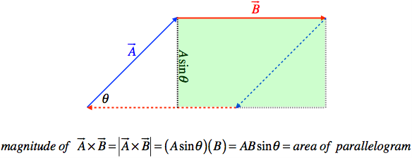
A nice consequence of this is that the magnitude of the cross product between 2 vectors become the area of the parallelogram formed by the two vectors. Neat!
Finally, we need to find a method to compute the cross product of 2 vectors.
Consider an arbitrary parallelogram Formed by 2 vectors inside a rectangular box
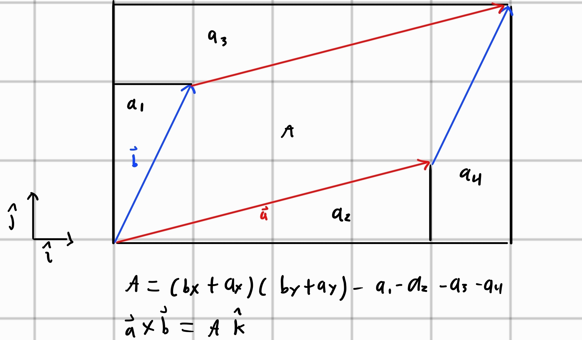
The area of this parallelogram will be denoted by \(A\). To find this area, we can take the total area of the rectangle and subract the other areas: \[A= (b_x+a_x)(b_y+a_y)-a_1-a_2-a_3-a_4\]
Using basic geometry, we can find that: \[a_1=\frac{b_x b_y}{2}\] \[a_2=\frac{a_x a_y}{2}\] \[a_3=\frac{a_y(2b_x+a_x)}{2}\] \[a_4=\frac{b_x(2a_y+b_y)}{2}\]
Plugging these into the equation for \(A\) and simplifying gives us that: \[A = a_x b_y - a_y b_x\]
Intuitively, as the vectors \(\vec{A}\) and \(\vec{B}\) are in the x-y plane, the cross product of them must point along the z axis, hence \[\vec{A} \times \vec{B} = (a_x b_y - a_y b_x)\hat{k}\]
We can repeat this process for the other 2 planes and combine them to get the full formula for the cross product of 2 vectors:
\[\vec{A} \times \vec{B} = (a_y b_z - a_z b_y)\hat{i} + (a_z b_x - a_x b_z)\hat{j} + (a_x b_y - a_y b_x)\hat{k}.\]Whoa, this formula is a bit hard to remember. Don't worry too much though, we will try to avoid using formulas as much as possible here, so we will very rarely be seeing this here.
That is the cross product. I've included an applet below to play around as the cross product may be a bit hard to visualize without a picture
Up next we have the dot product.
Dot product
This type of product generates a scalar and is denoted by \(\vec{A} \cdot \vec{B}\). While the cross product can be used to measure how perpendicular the vectors are, this one measures how aligned both vectors are. So instead of using the sine of the angle between them, we use the cosine of the angle between them to find the magnitude of the dot product. \[ \vec{A} \cdot \vec{B} = |\vec{A}||\vec{B}|\cos(\theta)\]
Use the applet above to experiment with it.
While the cross product is really only defined in 3d, we can see that the dot product is defined in any number of dimensions as it doesn't have a directional requirement.
To compute the dot product is far more straightforward than the cross product, as it simply involves multiplying the corresponding components of the vectors and summing them up:
\[\vec{A} \cdot \vec{B} = a_x b_x + a_y b_y + a_z b_z\]There we have it, the dot and cross products of vectors. These will be very useful in the following sections.
Back to rotations
Hm, We'll need to think about some counterpart to rotation. Imagine trying to close a door. We can easily see that the closer we are to the pivot when pushing the door it seems to be harder to rotate the door.
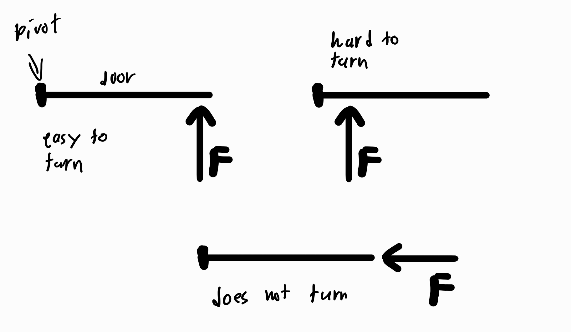
This hints that the rotational counterpart to force must be related to the force we exert along the rotational direction and the distance from the pivot which we exert the force from. The bottom figure here also shows that this "turning force" can only be generated when the force is applied perpendicular to the position from the pivot.
Because of this, we will define the rotational counterpart of the Force to be the torque, denoted by \(\vec{\tau}\). Torque is defined as the cross product of the position vector and the force vector:
\[\vec{\tau} = \vec{r} \times \vec{F}\]Where \(\vec{r}\) is the position vector from the axis of rotation to the point where the force is applied, and \(\vec{F}\) is the force vector.
Why the cross product? We use the cross product as we want to take the components of the force and displacement which are perpendicular to each other. Although torque seems to be a vector quantity, we call it a pseudovector as it doesn't interact with other physical vectors in the usual manner (check out geometric algebra for more details).
The magnitude of the torque can be calculated as:
\[|\vec{\tau}| = rF\sin(\theta)\]This turning force seems to make sense so far. But is it still consistent with Newton's second law? The short answer is yes, but it's a bit more complex than the linear version. In rotational dynamics, the analog of Newton's second law is:
\[\vec{\tau} = I\vec{\alpha}\]Where \(I\) is the moment of inertia and \(\vec{\alpha}\) is the angular acceleration. This equation seems to make sense as the angular force (torque) should be proportional to the angular acceleration. However, upon inspection, we have what is called the moment of inertia which seems to analogously correspond to mass in linear motion.
Just as force and torque are physically related, mass and moment of inertia are related in a similar way. The moment of inertia depends on the mass distribution of the object and the axis of rotation. Let's look into it a bit more to see their connection.
Moment of inertia
Consider a bob of mass \(m\) attached to a massless rod of length \(r\).
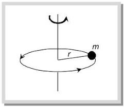
It's clear that if we tangentially exert a force \(\vec{F}\) on the bob, it should spin with some tangential acceleration. This acceleration is related to the radius by a factor of \(r\), so we have \[a_t = r\alpha.\] Using Newton's second law, we find that \[F = ma_t = mr\alpha.\] Substituting the torque equation, we get: \[\tau = rF = mr^2\alpha.\] This shows that the moment of inertia for a point mass is \(I = mr^2\).
That's neat and all, but what if we have a mass distribution or multiple point masses?
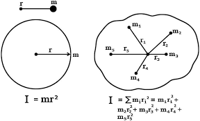
In such a case, similar to masses in a singular body, we can get the total moment of inertia for multiple point passes by summing them up: \[I = \sum_i m_i r_i^2.\] Where \(m_i\) is the mass of the \(i\)-th point mass and \(r_i\) is its perpendicular distance from the axis of rotation.
Similar to how we can obtain the total mass of a mass distribution by integrating the density over a volume, area or line, we can also obtain the moment of inertia for a continuous mass distribution by integrating the following: \[I = \int r^2 dm.\]Where \(dm\) is the infinitesimal mass element of the distribution.
This seems like an odd expression to have. What does it mean to integrate along masses? Recall that an integral along x is essentially a sum of the integrand multiplied by incriments of x.
So what this expression is saying is that we take small bits of mass from the distribution, multiply it by the square of its distance from the axis of rotation and sum them all up. This gives us the total moment of inertia for the mass distribution.
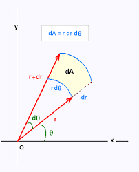
Using the chain rule, we can also express the integral as the following for more familiarity: \[ I = \int r^2 \sigma dA \]
Where \(\sigma=\frac{dm}{dA}\) is the surface mass density of the object and \(dA=dx dy\equiv r dr d\theta\) is the infinitesimal area element.
We can also use the linear mass density \(\lambda\) to express it as \[ I = \int r^2 \lambda dl \]
Where \(\lambda = \frac{dm}{dl}\) is the linear mass density and \(dl\) is the infinitesimal length element.
For example, let's try to find the moment of inertia of a rod of uniform mass density \(\lambda\) and a solid disc of uniform surface density \(\sigma\).
Example: Moment of inertia of a rod about its end
Consider a rod of length \(L\) and mass \(M\).
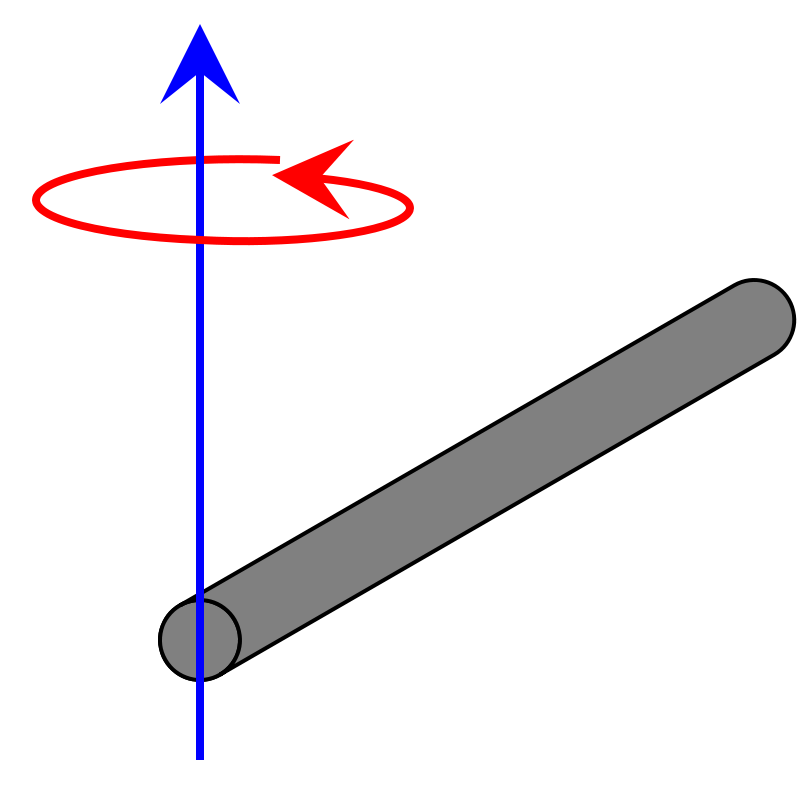
As the rod has uniform mass distribution, we can model the linear mass density as \(\lambda(r) = \frac{M}{L}\). It is independent of the position along the rod.
Now, we can make use of the integral expression for the moment of inertia along a line: \[I =\int r^2 dm = \int r^2 \lambda dr.\]
We then integrate along the length of the rod to find the moment of inertia: \[I = \int_0^L r^2 \lambda dr = \lambda \int_0^L r^2 dr = \lambda \left[ \frac{r^3}{3} \right]_0^L = \frac{\lambda L^3}{3} = \frac{M L^2}{3}. \]
Therefore, the moment of inertia of the rod about one end is \(\frac{1}{3}ML^2\).
Let's try something similar for the moment of inertia of the disc of mass M:
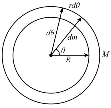
The disc will have uniform mass density, hence, we will find that \(\sigma = \frac{M}{\pi R^2}\), we then choose to set up the integral as:
\[I=\int r^2 dm=\int r^2 \sigma dA=\int_0^R \int_0^{2\pi} r^3 \sigma d\theta dr \]Performing the integrals sequentially and using the fact that \(\sigma = \frac{M}{\pi R^2}\) lets us find that the moment of inertia is given by:
\[I= \int_0^R r^3 \sigma\overbrace{\left[ \int_0^{2\pi} d\theta \right]}^{2\pi}dr= \int_0^R 2\pi r^3 dr=\left[\frac{\pi r^4}{2}\sigma\right]_0^R=\frac{1}{2}MR^2\]There we have it, the moment of inertia of a solid disc.
An interesting problem in Forces and Rotational Dynamics
Now that we've seen the 3 Laws of motion imposed by Newton and their rotational counterparts, let's see how we can apply them to solve problems in forces.
A big package: The Square atwood machine with slipping
Consider an atwood machine with a massless wheel of radius \(r\) holding the string connected to a solid square of mass M with side length s, the frictional coefficient which exerts a force \(F_f=_k F_n \) opposing the slipping of the string is given by \(\mu_k\) and the rope is wrapped around the wheel \(n\) times.
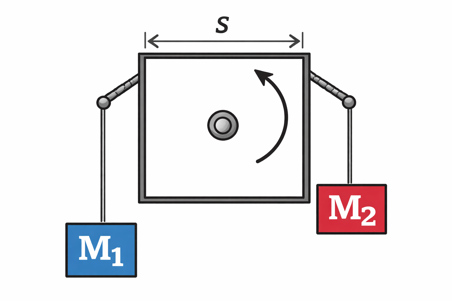
Find the equation of motion for the 2 blocks and the wheel in terms of the given variables.
Solution:
Hm, this seems like a really tough problem, the type that should scare physics students away due to the different things to take into consideration. Nevertheless, we will still try to do this problem step by step.
Let's start by first looking into the forces on each block here.
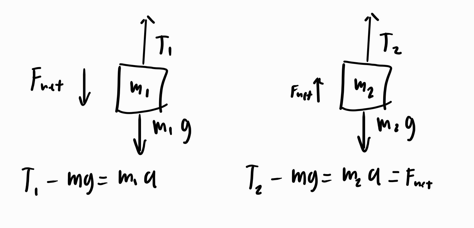
We will be assuming that block 2 accelerates up whilst block 1 drops. This may not be the case, but if this happens we will be getting a negative number for the acceleration, indicating that block 2 is accelerating up with a negative value which is equivalent to saying it is falling down.
We will now want to relate the 2 tensions \(T_2\) and \(T_1\) by looking into the friction on the wheel:
As the amount of frictional force on the string depends on the force which the string is exerting on the wheel, we will first have to find how much force is exerted onto the wheel as a function of the angle from either ends of the connection between the wheel and the string.
We can do so by looking into the tensions of the string at 2 points infinitesimally close to each other.
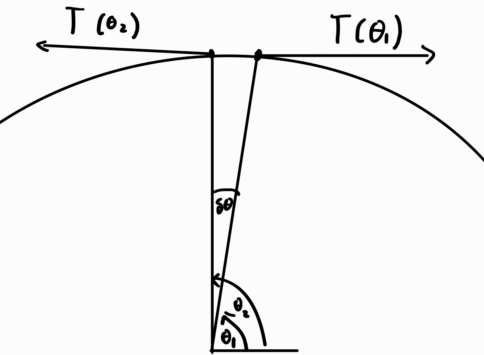
It's clear that the difference in magnitudes of the tensions in both points of the wheel must be related by the amount of friction around that point. Using this we can get the equation:
\[\delta T \approx \frac{dF_f}{d \theta}\delta \theta\]Where \(F_f\) is the frictional force at the angle \(\theta\).
We can also look into the force diagram and try to take the infinitesimal difference of the tension forces to get the normal force at the point
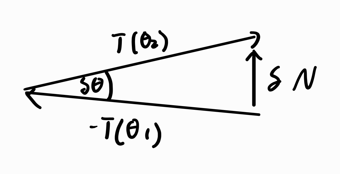
When the 2 angles get very close to each other, we can make the approximation \(T(\theta_2) \approx T(\theta_1)\), using a small angle approximation we can see that,
\[\delta N \approx T \delta \theta \]Where \(N\) is the normal force exerted by the string's tension.
Taking the limit as \(\delta \theta\) goes to \(0\) we find that we have 2 equations:
\[\frac{dN}{d\theta}(\theta)=T(\theta)\] \[\frac{dF_f}{d\theta}(\theta)=\frac{d T}{d\theta}(\theta)\]Making use of the fact that the frictional force is given by \(F_f=\mu_k N\), multiplying the first equation by a factor of \(\mu_k\) and combining both equations, we find that we will get the differential equation
\[\frac{d T}{d \theta}(\theta)=\mu T(\theta)\]To solve this differential equation we will use the exponential function. It is defined to be the function which is it's own derivative:
\[\frac{d}{dx}e^x=e^x\]Making use of the chain rule we will find that the solution of this equation will be given by:
\[T(\theta)=T(0) e^{\mu_k\theta}\]Now, if the string has N loops, we can find that the relationship between the tensions in the 2 ends to be (taking \(T_2\) to be \(T(0)\)) \(T_1=T_2 e^{\mu_k (2n+1)\pi}\), the extra \(\pi\) in the angle will be due to the fact that the 2 masses are on 2 opposite ends of the wheel but this detail isn't very important for the goal of the problem here (the picture was not very clear about it).
We are finally almost halfway through the problem. Now, equipped with the relationship between the tensions of the 2 ends, we can combine the equations to find that:
\[T_1-m_1g=m_1a\] \[T_2-m_2g=m_2a\] \[T_1=T_2 e^{\mu_k (2n+1)\pi}\]We now have 3 independent equations with 3 unknown variables (\(T_1,T_2,a\)). Solving this lets us find that the 2 blocks accelerates constantly with:
\[a = g \frac{m_1 - m_2 e^{\mu_k (2n+1)\pi}}{m_1 + m_2 e^{\mu_k (2n+1)\pi}}\]Nice! We've just finished the first half of this problem.
Now, we have to find how the block spins:
To do this, we simply need to remember Newton's 2nd law for rotation:
\[\tau=I \alpha\]We also have the equation,
\[|\tau|=|\vec{r}\times \vec{F}|.\]Which relates force to the torque applied onto he wheel. But what force are we using?
That would be the frictional force between the string and the wheel. We can find the frictional force by taking the difference in tension between the 2 ends of the atwood machine. Using some neat algebra, we find that,
\[F_f=T_2-T_1=\frac{2 m_1 m_2 g \left(1 - e^{\mu (2n+1)\pi}\right)}{m_1 + m_2 e^{\mu (2n+1)\pi}}.\]It's a pretty nasty expression, so we'll stick to using \(F_f\) as the frictional force, but at least we have an expression to use with our known quantities in disposal. Let's then draw a force diagram for this,
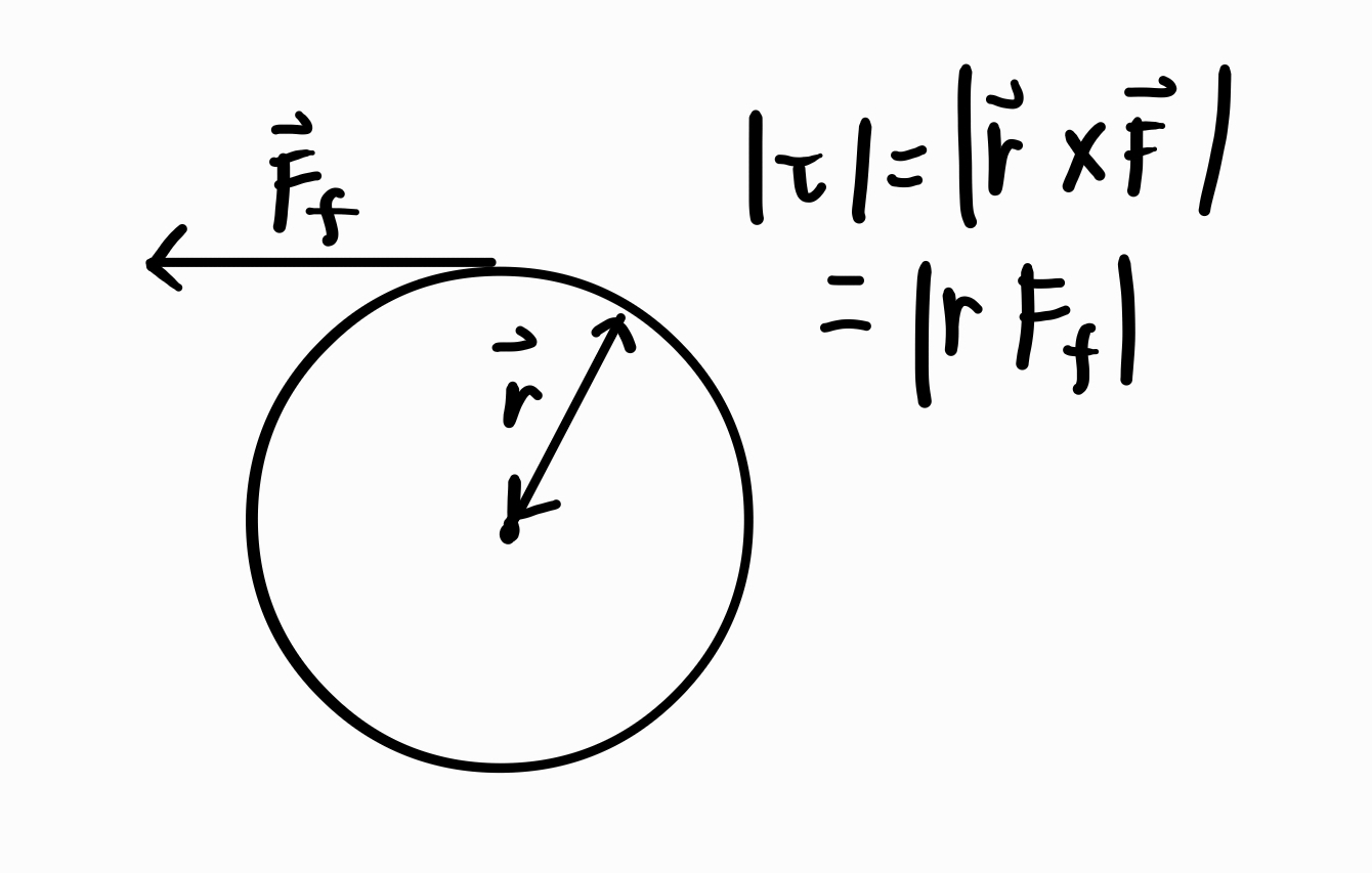
Now, we come back to the wheel here and take notice that the frictional force on the wheel is effective on the end of the wheel. Hence the equation of motion for the square and wheel becomes:
\[\tau=F_f r=(I_{square}+\overbrace{I_{wheel}}^0)\alpha\]We will want this equation of motion to be in terms of known quantities, so we'll try to exapnd the moment of inertia of the solid square in terms of our known quantities (M,s). Remember that the moment of inertia can be set up with the integral:
\[I=\int r^2 dm=\int r^2 \sigma dA \]Next, we'll want to think of how we can perform this area integral. Given that the object we are integrating is a square, it would seem to be appropriate to use cartesian coordinates(x,y) instead of the polar coordinates we used previously (\(r,\theta\)). So now our integral becomes:
\[I=\int r^2 \sigma(x,y) dA=\int_{-\frac{a}{2}}^{\frac{a}{2}} \int_{-\frac{a}{2}}^{\frac{a}{2}} (x^2+y^2)\sigma dx dy \]We have made \(\sigma(x,y)\) a constant as the solid square has uniform mass density. Performing the integrals sequantially, we can find that the moment of inertia becomes:
\[I=\int_{-\frac{a}{2}}^{\frac{a}{2}}\overbrace{\left[ \frac{x^3}{3} + xy^2 \right]_{x=-\frac{a}{2}}^{x=\frac{a}{2}}}^{\frac{a^3}{12} + ay^2} \sigma dy= \int_{-\frac{a}{2}}^{\frac{a}{2}} (\frac{a^3}{12} + ay^2)\sigma dy = \frac{\sigma a^4}{6}\]Now, we make use of the fact that the mass of the square is \(M\) to find that \(\sigma=\frac{M}{a^2}\) and simplify the moment of inertia to be:
\[I=\frac{Ma^2}{6}.\]Then we go back to the equation of motion for the square to find that
\[\alpha=\frac{\tau}{I}=\frac{F_f r}{I}= \frac{12 m_1 m_2 g r \left(1 - e^{\mu (2n+1)\pi}\right)}{M a^2 \left(m_1 + m_2 e^{\mu (2n+1)\pi}\right)}.\]That is the problem solved!
This may seem very difficult, but don't worry too much, the main point isn't to be able to juggle all these different variables it was just to see how powerful these concepts can be when put together with some maths. This was a problem I though up of when I was commuting in a train (They usually come out to be very nasty).
That is all I have for forces for now. Next up, we have energy.